Amazon Redshift Distribution vs Partitioning: Why Redshift Has No PARTITION BY (and What to Use Instead)
If you're learning AWS Redshift after PostgreSQL or Hive, the missing PARTITION BY clause is confusing. Here's how DISTKEY, SORTKEY, and zone maps replace partitioning in an AWS data lake and data warehouse — with side-by-side SQL examples.
If you come to Amazon Redshift from PostgreSQL, MySQL, Oracle, or BigQuery, one of the first things that trips you up is this:
CREATE TABLE orders (...)
PARTITION BY RANGE (order_date);   -- ❌ Syntax error in Redshift
Redshift doesn't support PARTITION BY. And it's not an oversight — AWS calls this out explicitly in the Redshift docs:
"Amazon Redshift does not require or support the concept of partitioning data within database objects. There's no need to partition databases or tables."
That sentence confuses a lot of people learning AWS data lake and data warehouse patterns for the first time. If partitioning is the standard tool for making big tables fast, how can a modern cloud data warehouse just… not have it?
The short answer: Redshift solves the same two problems partitioning solves, but with two different mechanisms. Once you see what those two problems actually are, the whole Redshift design — DISTKEY, SORTKEY, slices, zone maps — clicks into place.
This post is for engineers, data analysts, and bootcamp learners trying to make that mental leap.
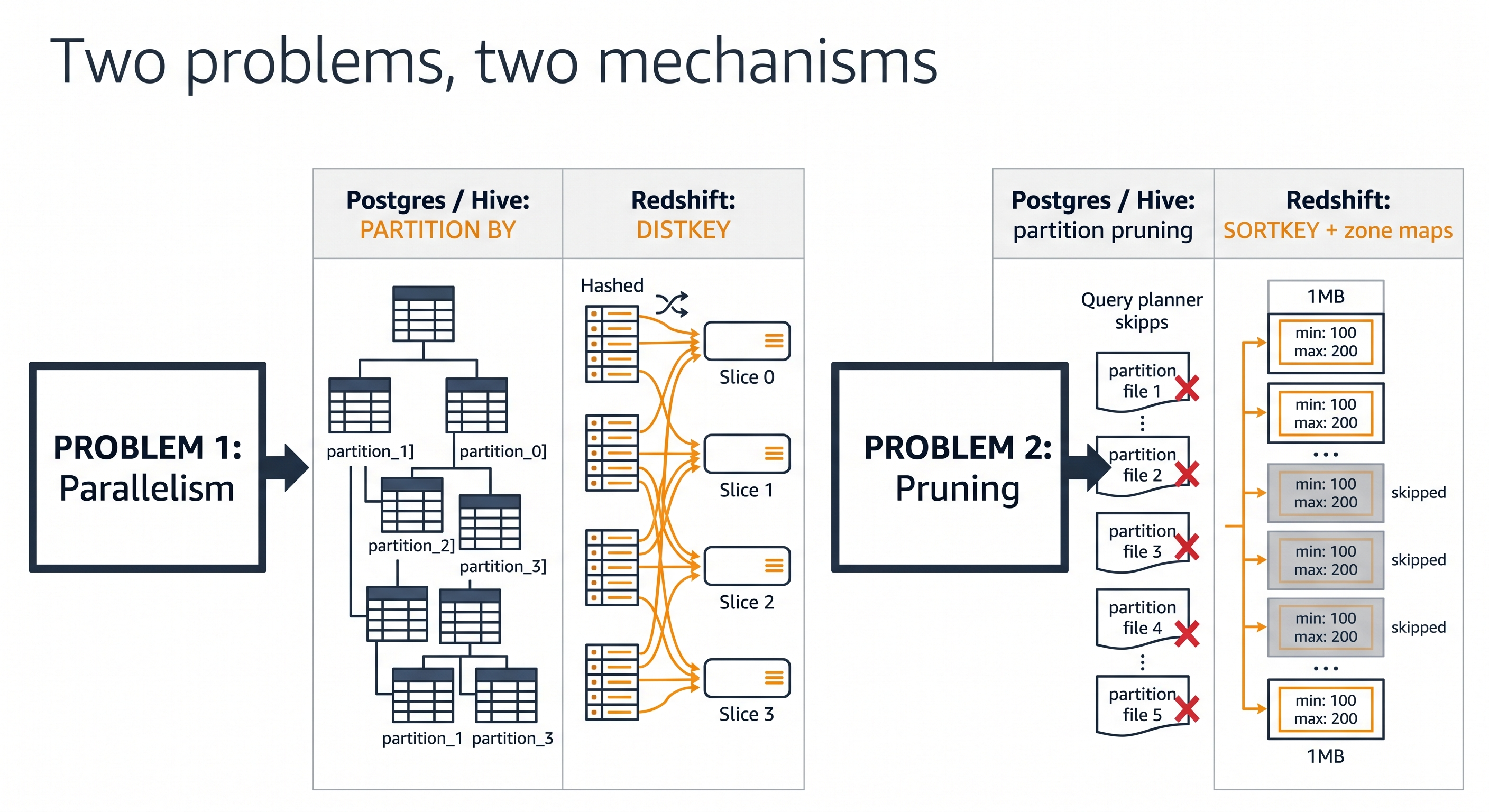
The Two Problems Partitioning Tries to Solve
Whenever you reach for PARTITION BY in another database, you're really trying to fix one (or both) of these:
- Parallelism — "I have 200M rows. I want N workers to scan their slice of the table at the same time."
- Pruning — "My query only touches
order_date >= '2025-01-01'. I don't want to read the other 364 days off disk."
Most engines bundle both jobs into the partition definition. You write PARTITION BY RANGE (order_date) and that single clause decides which physical chunk a row lives in and which chunks the planner can skip.
Amazon Redshift unbundles them.
| Problem | Postgres / Hive / BigQuery answer | Amazon Redshift answer |
|---|---|---|
| Parallelism — spread work across workers | Partitions + partition-aware scans | DISTKEY (or AUTO / EVEN / ALL) places rows on slices |
| Pruning — skip data you don't need to read | Partition pruning by partition column | SORTKEY + zone maps skip 1MB blocks whose min/max don't match the predicate |
Two problems, two knobs. They're independent — you can pick a DISTKEY for join performance and a totally unrelated SORTKEY for filter performance, and they won't interfere with each other.
How Other Database Systems Compare
If you're moving between cloud data warehouses and lakehouses, this comparison is worth pinning to the wall:
| System | Has partitions? | Primary parallelism mechanism | Primary pruning mechanism |
|---|---|---|---|
| PostgreSQL | Yes — declarative PARTITION BY | Partition-wise scans | Partition pruning |
| Hive / Spark on S3 | Yes — Hive-style folder partitions | One task per partition file | Folder-level partition pruning |
| Google BigQuery | Yes — partitioned + clustered tables | Slot-based; partitions help | Partition pruning + clustering |
| Snowflake | No (uses micro-partitions, automatic) | Micro-partition fan-out | Micro-partition metadata |
| Amazon Redshift | No | DISTKEY → slices | SORTKEY + zone maps |
Snowflake and Redshift are actually closer to each other than either is to Postgres: both hide the physical layout from you and ask you to express intent (distribute by this, sort by that) instead of layout (put rows in this file). This is a defining trait of modern cloud-native data warehouses.
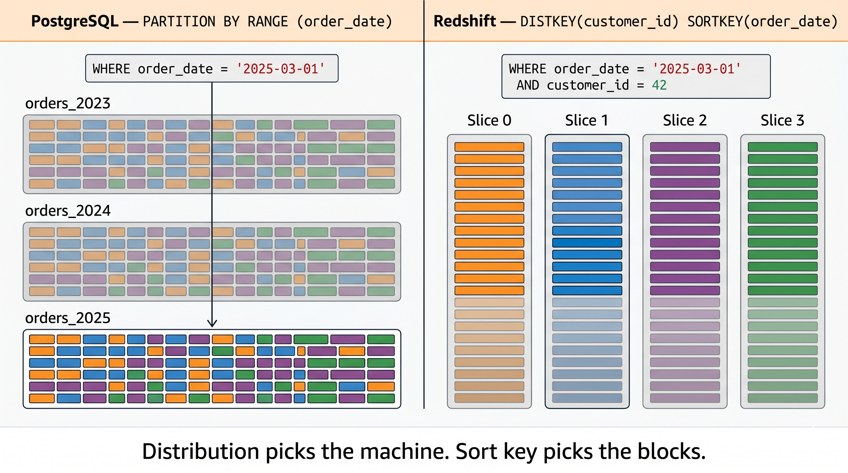
Side-by-Side Example: PostgreSQL Partitioning vs Redshift DISTKEY + SORTKEY
Take a classic orders table. You want fast filters by date and fast joins to customers.
PostgreSQL — partition the table
CREATE TABLE orders (
    order_id    BIGINT,
    customer_id BIGINT,
    order_date  DATE,
    amount      NUMERIC(10,2)
)
PARTITION BY RANGE (order_date);

CREATE TABLE orders_2024 PARTITION OF orders
    FOR VALUES FROM ('2024-01-01') TO ('2025-01-01');

CREATE TABLE orders_2025 PARTITION OF orders
    FOR VALUES FROM ('2025-01-01') TO ('2026-01-01');

CREATE INDEX ON orders (customer_id);
Result: physical files split by year. Filtering by order_date prunes whole files. Joins on customer_id use a B-tree index.
Amazon Redshift — distribute and sort
CREATE TABLE orders (
    order_id    BIGINT,
    customer_id BIGINT,
    order_date  DATE,
    amount      NUMERIC(10,2)
)
DISTKEY (customer_id)      -- rows with the same customer_id co-locate on one slice
SORTKEY (order_date);      -- within each slice, rows are stored in date order
Result: rows hashed across slices by customer_id (so a join to customers DISTKEY(customer_id) is a local join, no shuffle). Within every slice, rows sit in date order, and zone maps on each 1MB block let the planner skip blocks whose date range doesn't match.
Notice what we got:
- Same parallelism story as partitioning — work is spread across N workers — but the unit is a slice, not a partition file.
- Same pruning story as partitioning — irrelevant data isn't read — but the unit is a 1MB block, not a partition.
- Plus something partitioning can't easily give you: co-located joins. You only get this in Postgres if both tables are partitioned identically and the planner cooperates.
DISTKEY vs SORTKEY vs Partitioning — A Detailed Comparison
| Aspect | Partitioning (Postgres / Hive / BigQuery) | Redshift Distribution + Sort |
|---|---|---|
| Declared in DDL? | Yes — PARTITION BY ... | Yes — DISTKEY(...) + SORTKEY(...) |
| Granularity | Coarse — usually one partition per day/month/region | Fine — 1MB blocks, automatic |
| Storage layout | One file/segment per partition | One column file per slice; blocks within |
| Pruning mechanism | Planner reads partition metadata, skips files | Planner reads zone map (min/max per block), skips blocks |
| Parallelism unit | Partition | Slice (fixed per node, e.g. 2 per ra3.xlplus) |
| Maintenance burden | Add new partitions, drop old ones, repartition on schema change | None — sort order maintained by VACUUM; AUTO can choose for you |
| Join co-location | Only if both tables partitioned the same way | Yes — same DISTKEY = local join, no network shuffle |
| Goes wrong when… | Wrong partition column, or too many/few partitions | Wrong DISTKEY (skew) or wrong SORTKEY (no pruning) |
The maintenance row is the one most engineers undersell. With Hive-style partitions on S3, picking the wrong partition column at table-creation time is a multi-day rebuild. With Redshift, you can ALTER TABLE ... ALTER DISTKEY or ALTER SORTKEY and let the system reorganize in the background. This is one of the underrated advantages of a managed cloud data warehouse.
The Redshift Mental Model in One Sentence
Distribution decides which machine a row lives on. Sort key + zone maps decide which blocks the engine bothers to read. Partitioning conflates the two into a single, coarser knob.
If you internalize that one line, every Redshift performance decision gets easier:
- "My join is slow." → Look at DISTKEY. Are the two tables co-located? Is there data skew across slices?
- "My filter is slow." → Look at SORTKEY. Does it match the predicate? Has
ANALYZEbeen run recently? - "One slice is doing all the work." → Bad DISTKEY. You probably hashed on a low-cardinality column.
- "Zone maps aren't helping." → SORTKEY doesn't match your filter columns, or the table needs a
VACUUM.
In Postgres, all of those symptoms have a single suspect: "did I partition this right?" In Redshift, the suspects are split — and that's a feature, not a bug.
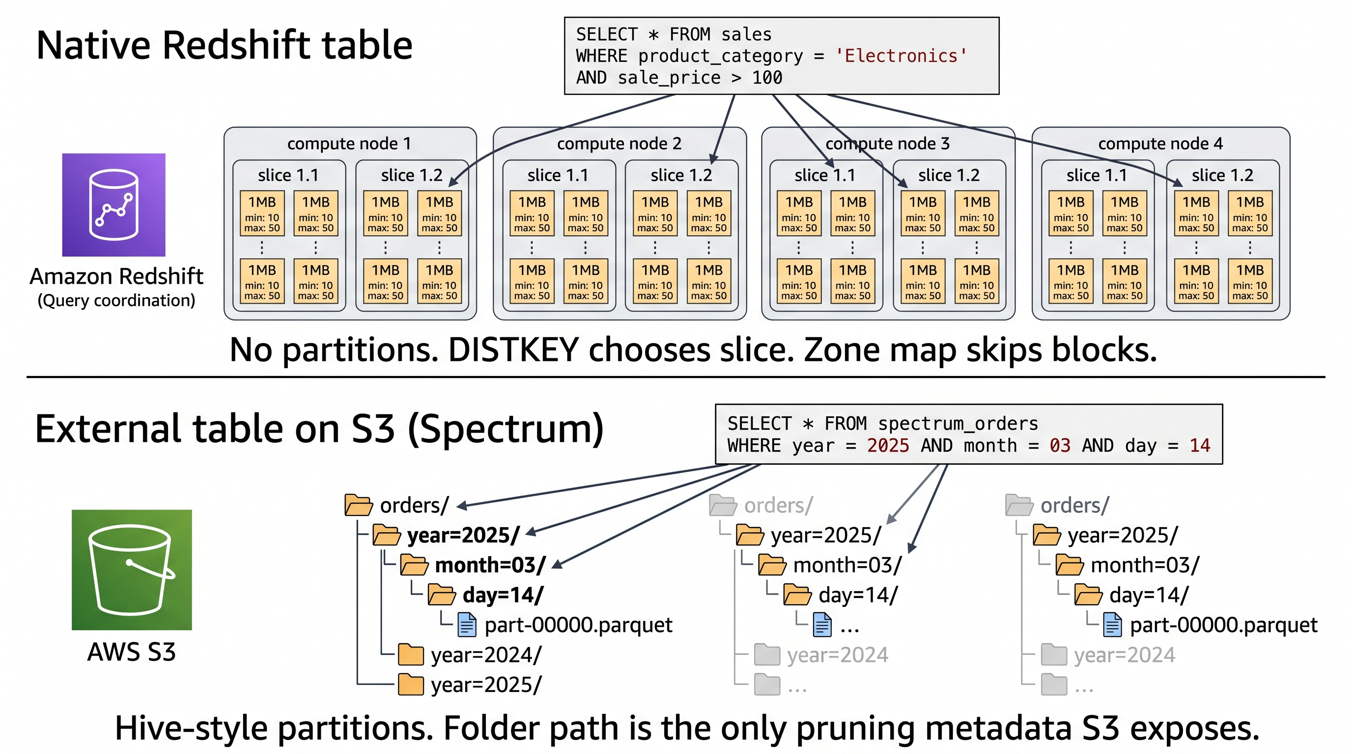
Where Partitioning Does Show Up in the AWS Data Lake World
There's one big exception worth knowing: external tables in Redshift Spectrum, Athena, and AWS Glue. When Redshift reads Parquet files on Amazon S3, it uses Hive-style folder partitions:
s3://lake/orders/year=2025/month=03/day=14/part-00000.parquet
CREATE EXTERNAL TABLE spectrum.orders (
    order_id    BIGINT,
    customer_id BIGINT,
    amount      DECIMAL(10,2)
)
PARTITIONED BY (year INT, month INT, day INT)
STORED AS PARQUET
LOCATION 's3://lake/orders/';
This is Hive-style partition pruning, and it works exactly like it does in Apache Spark or Athena. The reason it exists here and not for native Redshift tables is that S3 has no zone maps — the only metadata available is the folder path. Partitioning is how you bolt pruning onto a filesystem that doesn't have it natively.
So the full picture for engineers building on AWS:
- Native Redshift tables on cluster storage → no partitions. Use DISTKEY + SORTKEY.
- External tables on S3 (Spectrum, Athena, Glue) → partitions, because that's the only pruning mechanism Parquet-on-S3 offers. (Iceberg metadata is starting to change this, but partitioning is still the cheap, universally supported path.)
This is the same split you see in a typical modern AWS data lake architecture: hot, low-latency analytics on Redshift native storage; cheap, scalable historical data on S3 via Spectrum.
Practical Takeaway for Engineers Migrating to Redshift
If you're moving a workload from PostgreSQL, MySQL, or Hive to Amazon Redshift, the migration question isn't "what's the equivalent partition?" — it's "what are the two things my partition column was doing for me?" Then map each one separately:
- The "spread work across workers" job → DISTKEY (usually your largest join key).
- The "skip irrelevant rows" job → SORTKEY (usually your most common filter column — often a date or timestamp).
Most of the time, those are different columns. That's the part partitioning hides from you, and the part Redshift makes you confront. Once you see them as separate decisions, you'll write better DDL on every engine you touch — including the ones that still call them partitions.
If you're learning Redshift as part of a broader AWS data lake or data engineering path, this is one of the highest-leverage mental models you can build early. Get this right, and the rest of the Redshift performance toolkit — VACUUM, ANALYZE, AUTO distribution, materialized views, concurrency scaling — becomes a much shorter list to learn.
Further Reading
- Choosing a data distribution style — AWS Redshift Docs
- Columnar storage in Amazon Redshift — AWS Docs
- Amazon Redshift Best Practices for Designing Tables (source of the "no partitioning" quote)
- Querying external data using Amazon Redshift Spectrum
If you're working through Redshift and AWS data lake concepts as part of a structured learning path, our bootcamp programs cover these design decisions hands-on with real datasets — including the trade-offs between DISTKEY choices, sort key strategies, and when to push workloads into Spectrum vs keep them on native storage.